SAS Data Analysis

Part I: Descriptive Statistics 

1. Using the data set IRIS in the SASHELP library, generate summary statistics for the variables PetalLength and PetalWidth. Include the mean, standard deviation, median, the number of non-missing observations, and the number of missing observations. Then Make a histogram of the variable _PetalLength and describe its distribution. 

proc means data=SASHELP.IRIS chartype mean std median n nmiss vardef=df 

qmethod=os;

var PetalLength PetalWidth;

run;

proc univariate data=SASHELP.IRIS vardef=df noprint;

var PetalLength PetalWidth;

histogram PetalLength PetalWidth / normal(noprint);

run;

Variable	Label	Mean	Std Dev	Median	N	N Miss
PetalLengthPetalWidth	Petal Length (mm)Petal Width (mm)	37.580000011.9933333	17.65298237.6223767	43.500000013.0000000	150150	00

From the histogram, we can see that the distribution of values doesn’t follow the normal curve very well. It is a non-normally distributed variable of PetalLength.

2. Using the same dataset in question 1, check for normality for the variable PetalLength. Add a Normal Quantile-Quantile (Q-Q) plot and compute the sample skewness for the variable. 

proc univariate data=sashelp.iris normal plot;

var petallength;

qqplot petallength /normal(mu=est sigma=est color=red l=1);

run;

proc freq;

tables species/chisq;

run;

We can see that the data points near the tails and heads don’t fall exactly along a straight line. We can see the clear departure from the straight line in this Q-Q plot, indicating that this dataset likely does not follow a normal distribution.

Tests for Normality
		Test	Statistic	p Value
Shapiro-Wilk	W	0.876268	Pr < W	<0.0001
Kolmogorov-Smirnov	D	0.198154	Pr > D	<0.0100
Cramer-von Mises	W-Sq	1.222285	Pr > W-Sq	<0.0050
Anderson-Darling	A-Sq	7.678546	Pr > A-Sq	<0.0050

According to SAS Manual (Sas.com, 2023), if the sample size is less than 2000, the Shapiro test is better. Since the p-value for each normality test is less than 0.05, we would reject the null hypothesis for each normality test. This means there is sufficient evidence to conclude that the points variable is not normally distributed.

The UNIVARIATE Procedure

Variable: PetalLength (Petal Length (mm))

			Moments
N	150	Sum Weights	150
Mean	37.58	Sum Observations	5637
Std Deviation	17.6529823	Variance	311.627785
Skewness	-0.2748842	Kurtosis	-1.4021034
Uncorrected SS	258271	Corrected SS	46432.54
Coeff Variation	46.9744075	Std Error Mean	1.44135997

The variable PetalLength shows a negative value of skewness (-0.27) which indicates that the data is skewed to the left.

3. Using the same data as in exercise 1, compute the one-way table of the frequencies for the variable Species. 

proc freq data=SASHELP.IRIS;

tables Species / plots=(freqplot cumfreqplot);

Run;

The FREQ Procedure

				Iris Species
Species	Frequency	Percent	CumulativeFrequency	CumulativePercent
Setosa	50	33.33	50	33.33
Versicolor	50	33.33	100	66.67
Virginica	50	33.33	150	100.00

4. Using the same dataset, generate a box-plot for the variable PetalLength using Species as the category variable. Remove the species Virginica from the data presented in the boxplot.

data work.filter;

set sashelp.iris;

where Species in (‘Setosa’, ‘Versicolor’);

run;

proc print data=work.filter;

ods graphics / reset width=6.4in height=4.8in imagemap;

proc sgplot data=WORK.FILTER;

vbox PetalLength / category=Species;

yaxis grid;

run;

ods graphics / reset;

• The middle line of box Setosa lies outside of box Versicolor entirely. Then there is likely to be a difference between PetalLength in Setosa and Petal Length in Versicolor. 

• Petal Length in Sentosa is comparatively short than in Versicolor which is comparatively tall and it is an obvious difference between Setosa and Versicolor which is worthy for further investigations. 

• The box plot for petal length in Setosa is much lower than the equivalent plot for Versicolor and it is shoerter boz which mean their data points consistently hover around the center values. 

• The boxplot for petal length in Versicolor however has a longer whisker which indicates the larger range, more variable data  and wider distribution (more scattered data). 

• The outliers (the dotted outside the whiskers) in Setosa and Versicolor is about 1.5 times the size of the boxes.

• Setosa box is completely below Versicolor box which indicates there is a difference between the two group.

Part II: One-sample Tests 

1. Using the data set Heart in the SASHELP library, use a one-way t-test to determine if the mean weight of the population from which the sample was drawn is equal to 150 lbs. Include a test of normality and generate a histogram and box-plot. Should you be concerned that the test for normality rejects the hypothesis at the 0.05 significance level? 

proc ttest data=sashelp.heart h0=150 plots(showh0) alpha=0.05;

   var weight;

run;

The TTEST Procedure

Variable: Weight

N	Mean	Std Dev	Std Err	Minimum	Maximum
5203	153.1	28.9154	0.4009	67.0000	300.0

		Mean	95% CL Mean	Std Dev	95% CL Std Dev
153.1	152.4	153.9	28.9154	28.3704	29.4820

DF	t Value	Pr > t
5202	7.70	<.0001

Since the p-value (t = 7.7, p = <.0001) is less than .05, we reject the null hypothesis. This means we have sufficient evidence to say that the mean weight of the population from which the sample was drawn is different than 150 lbs.

The histogram above shows the overlaid normal and kernel densities, a box plot, the 95% confidence interval for the mean, and the null value of 150 lbs. The confidence interval excluded the null value, consistent with the rejection of the null hypothesis at alpha = 5%.

The curvilinear shape of the Q-Q plot suggests a possible slight deviation from normality. 

proc univariate data=sashelp.heart normal plot;

var weight;

qqplot weight /normal(mu=150 sigma=est color=red l=1);

run;

proc freq;

tables weight/chisq;

run;

Tests for Normality
		Test	Statistic	p Value
Kolmogorov-Smirnov	D	0.048465	Pr > D	<0.0100
Cramer-von Mises	W-Sq	3.05329	Pr > W-Sq	<0.0050
Anderson-Darling	A-Sq	18.50518	Pr > A-Sq	<0.0050

Since the p-value for each normality test is less than .05, we would reject the null hypothesis for each normality test. This means there is sufficient evidence to conclude that the points variable is not normally distributed, which confirms the histogram and Q-Q plots.

The UNIVARIATE Procedure

Variable: Weight

			Moments
N	5203	Sum Weights	5203
Mean	153.086681	Sum Observations	796510
Std Deviation	28.9154261	Variance	836.101866
Skewness	0.55594115	Kurtosis	0.52275608
Uncorrected SS	126284474	Corrected SS	4349401.91
Coeff Variation	18.8882703	Std Error Mean	0.40086919

The variable Weight shows a positive value of skewness (0.55) which indicates that the data is skewed to the right (right-skewed distribution), which confirm the histogram chart and Q-Q Plot.

Part III: Two-sample tests 

1. Using the Heart data in the SASHELP library, compare the Systolic (systolic blood pressure) for males and females (variable Sex indicate gender where values F and M indicates gender female respectively male. Generate a histogram and box-plot to investigate the distribution of Systolic for males and females. Can we assume that these are normal distributed based the histogram? 

proc means data=SASHELP.HEART chartype mean std median n nmiss vardef=df 

qmethod=os;

var Systolic;

class Sex;

run;

proc univariate data=SASHELP.HEART vardef=df noprint;

var Systolic;

class Sex;

histogram Systolic / normal(noprint);

run;

						Analysis Variable : Systolic
Sex	N Obs	Mean	Std Dev	Median	N	N Miss
Female	2873	136.8861817	25.9835883	130.0000000	2873	0
Male	2336	136.9383562	20.6535522	134.5000000	2336	0

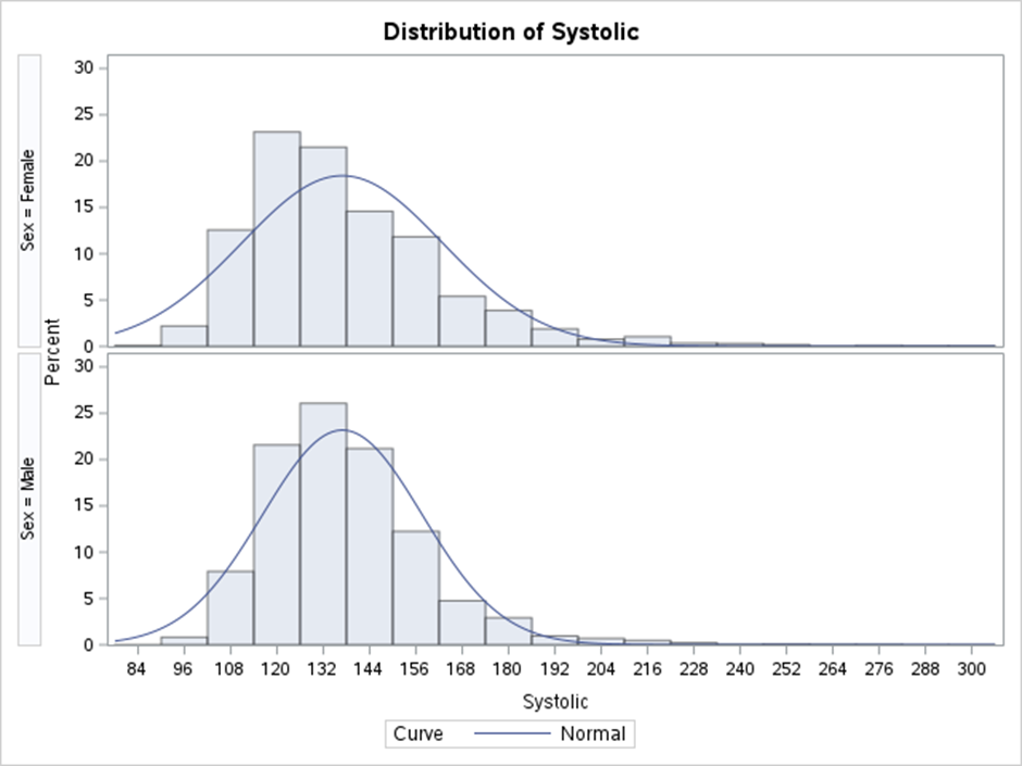
From the histogram, we can see that both Systolic in Male and Female are slightly right-skewed as it has tail on the right side of the distribution. This type of distribution is positively skewed distribution and non-normal distributed.

proc sgplot data=SASHELP.HEART;

vbox Systolic / category=Sex;

yaxis grid;

run;

ods graphics / reset;

• 
  

  

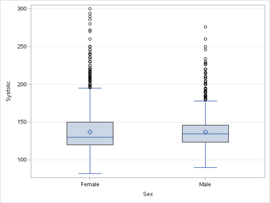
  The Systolic Male and Systolic Femal boxes are overlap wth one another which indicates the group is not much different. 

• The middle line of Systolic in Female box is slightly lower than the middle line of Systolic Male box. Then there is likely to be a difference between Systolic in female and male. 

• The box plot for Systolic in Male is shorter than Systolic Female box, which mean their data points consistently hover around the center values. 

• The boxplot for Systolic in Female is taller box and has a longer whisker which indicates the larger range, more variable data and wider distribution (more scattered data). 

• The outliers (the data points dotted outside the whiskers) in Systolic in Female and Male are above the box and are about 1.2 times the size of the boxes.

proc sgplot data=SASHELP.HEART;

  vbox Systolic / group=sex;

  keylegend / title=”Systolic for Males and Females”;

run;

• 

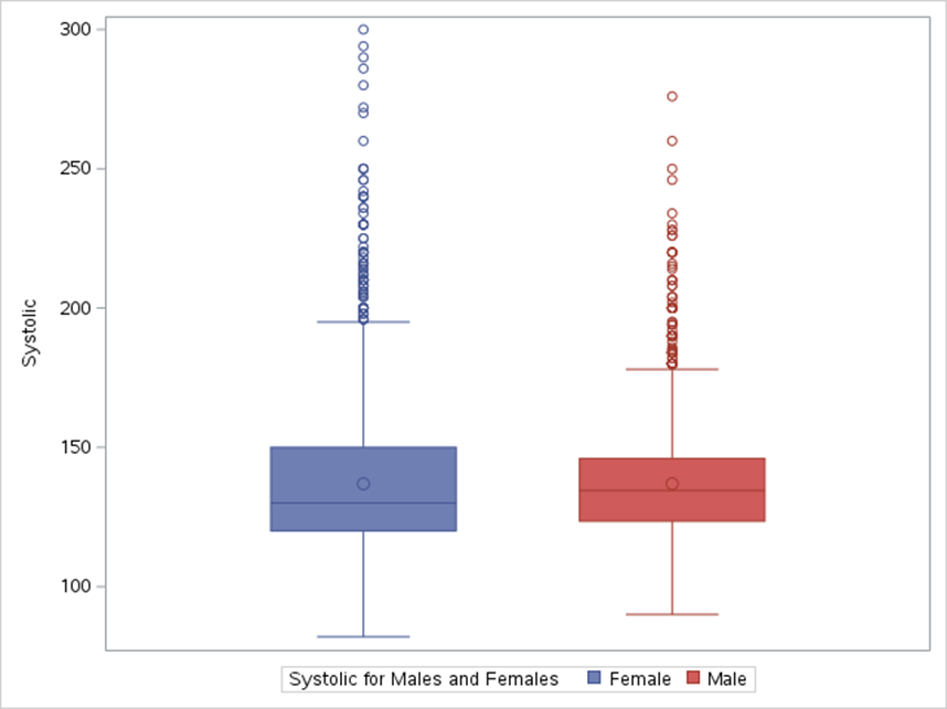
• The Median Values: The line in the middle of the box plot for Male is higher than the line for Female, which indicated that the gender Male had a higher median systolic.

• The Dispersion: The box plot for Female is slightly longer than Male, which indicates that the Systolic are much more spread out among Female.

• The Skewness: The line in the middle of the box plot for Male is at the center of the box, which indicates that the distribution of Systolic has little skew at all. 

2. Conduct the tests for normality. Do you reject the null hypothesis that the data values are normally distributed? 

proc univariate data=sashelp.heart normal;

var systolic;

class sex;

run;

Variable: Systolic

Sex = Female

			Moments
N	2873	Sum Weights	2873
Mean	136.886182	Sum Observations	393274
Std Deviation	25.9835883	Variance	675.14686
Skewness	1.51582354	Kurtosis	3.98506675
Uncorrected SS	55772798	Corrected SS	1939021.78
Coeff Variation	18.9818928	Std Error Mean	0.48476506

Basic Statistical Measures
		Location	Variability
Mean	136.8862	Std Deviation	25.98359
Median	130.0000	Variance	675.14686
Mode	120.0000	Range	218.00000
		Interquartile Range	30.00000

Tests for Location: Mu0=0
		Test	Statistic	p Value
Student’s t	t	282.3763	Pr > |t|	<.0001
Sign	M	1436.5	Pr >= |M|	<.0001
Signed Rank	S	2064251	Pr >= |S|	<.0001

Tests for Normality
		Test	Statistic	p Value
Kolmogorov-Smirnov	D	0.124774	Pr > D	<0.0100
Cramer-von Mises	W-Sq	10.35425	Pr > W-Sq	<0.0050
Anderson-Darling	A-Sq	60.9063	Pr > A-Sq	<0.0050

• Since the p-value for each normality test is less than .05, we would reject the null hypothesis for each normality test.

• This means there is sufficient evidence to conclude that the Systolic in Female variable is not normally distributed.

	Quantiles (Definition 5)
Level	Quantile
100% Max	300
99%	230
95%	185
90%	170
75% Q3	150
50% Median	130
25% Q1	120
10%	110
5%	106
1%	98
0% Min	82

Extreme Observations
		Lowest	Highest
Value	Obs	Value	Obs
82	554	280	2726
86	1125	286	4173
89	2425	290	5099
90	4829	294	3251
90	3236	300	4629

Variable: Systolic

Sex = Male

			Moments
N	2336	Sum Weights	2336
Mean	136.938356	Sum Observations	319888
Std Deviation	20.6535522	Variance	426.569218
Skewness	1.33026148	Kurtosis	3.6509985
Uncorrected SS	44800976	Corrected SS	996039.123
Coeff Variation	15.0823719	Std Error Mean	0.42732504

Basic Statistical Measures
		Location	Variability
Mean	136.9384	Std Deviation	20.65355
Median	134.5000	Variance	426.56922
Mode	140.0000	Range	186.00000
		Interquartile Range	22.50000

Tests for Location: Mu0=0
		Test	Statistic	p Value
Student’s t	t	320.4548	Pr > |t|	<.0001
Sign	M	1168	Pr >= |M|	<.0001
Signed Rank	S	1364808	Pr >= |S|	<.0001

Tests for Normality
		Test	Statistic	p Value
Kolmogorov-Smirnov	D	0.117447	Pr > D	<0.0100
Cramer-von Mises	W-Sq	5.452689	Pr > W-Sq	<0.0050
Anderson-Darling	A-Sq	32.9541	Pr > A-Sq	<0.0050

• Since the p-value for each normality test is less than .05, we would reject the null hypothesis for each normality test.

• This means there is sufficient evidence to conclude that the Systolic in Male variable is not normally distributed.

	Quantiles (Definition 5)
Level	Quantile
100% Max	276.0
99%	204.0
95%	174.0
90%	162.0
75% Q3	146.0
50% Median	134.5
25% Q1	123.5
10%	114.0
5%	110.0
1%	102.0
0% Min	90.0

Extreme Observations
		Lowest	Highest
Value	Obs	Value	Obs
90	2495	234	3115
94	5209	246	3608
94	4821	250	3574
96	5078	260	3953
96	4549	276	3598

• The variable Systolic in Female and Male show positive value of skewness (1.52 and 1.33), which indicates that the data is skewed to the right (right-skewed distribution), which confirm the histogram chart and Q-Q Plot that the data do not follow a normal distribution.

  

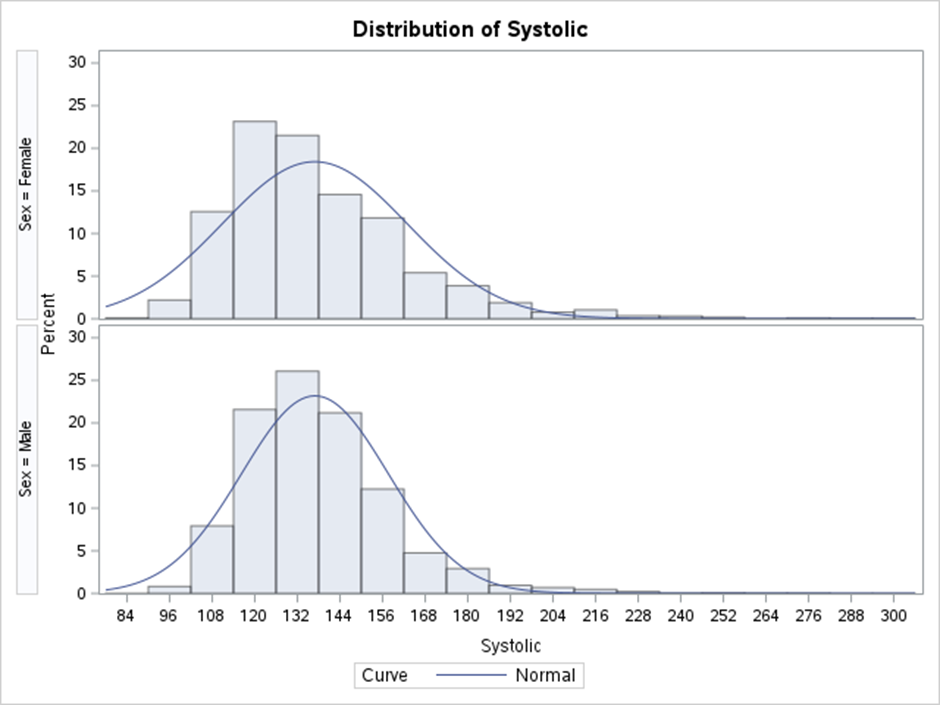
• From the histogram we can see that the distribution of Systolic in Male and Systolic in Female don’t follow the normal curve very well, which agrees with the results of the normality tests that we performed.

3. Run a two-sample t-test comparing the Systolic (systolic blood pressure) for males and females where Ho states that the difference in population means is zero (use 1 % significance level). Can we assume equal variances for men and females? 

proc ttest data=sashelp.heart h0=0 plots(showh0) alpha=0.01;

  var systolic;

  class sex;

run;

The TTEST Procedure

Variable: Systolic

Sex	Method	N	Mean	Std Dev	Std Err	Minimum	Maximum
Female		2873	136.9	25.9836	0.4848	82.0000	300.0
Male		2336	136.9	20.6536	0.4273	90.0000	276.0
Diff (1-2)	Pooled		-0.0522	23.7419	0.6614
Diff (1-2)	Satterthwaite		-0.0522		0.6462

		Sex	Method	Mean	99% CL Mean	Std Dev	99% CL Std Dev
Female		136.9	135.6	138.1	25.9836	25.1277	26.8955
Male		136.9	135.8	138.0	20.6536	19.9016	21.4604
Diff (1-2)	Pooled	-0.0522	-1.7565	1.6522	23.7419	23.1564	24.3556
Diff (1-2)	Satterthwaite	-0.0522	-1.7173	1.6130

				Equality of Variances
Method	Num DF	Den DF	F Value	Pr > F
Folded F	2872	2335	1.58	<.0001

• The ratio of variances is 1.58 indicating that the two groups have similar sample variances and thus we might assume that they have equal population variances for male and females. 

• The Equality of Variances test reveals sufficient evidence of unequal variances and is significant (Pr>F = .0001, with p=.0001), so we reject the null hypothesis of equal population variances. In this case, the variances appear to be unequal.

Method	Variances	DF	t Value	Pr > |t|
Pooled	Equal	5207	-0.08	0.9371
Satterthwaite	Unequal	5204.4	-0.08	0.9357

• In the t-test table above we choose Satterthwaite t-test (Unequal variances), and report a t statistic is -0.08 with 5204.4 degrees of freedom, with p-value of p=0.9357. Since p-value is greater than .1, we fail to reject the null hypothesis of equal population variances for males and females. 

• We can assume equal variances for males and females at 1 % significance level.

Part IV: Linear Regression Analysis 

1. Using the Cars dataset in the SASHELP library, run a multiple regression with MSRP as the dependent variable and the three variables Horsepower, Weight, and Length as the predictor variables. Interpret the results. Is there evidence of multicollinearity?

proc reg data=sashelp.cars;

model msrp = horsepower weight length;

Run;

The REG Procedure

Model: MODEL1

Dependent Variable: MSRP

Number of Observations Read	428
Number of Observations Used	428

					Analysis of Variance
Source	DF	Sum ofSquares	MeanSquare	F Value	Pr > F
Model	3	1.141437E11	38047899508	342.60	<.0001
Error	424	47087920181	111056416
Corrected Total	427	1.612316E11

• The overall F-value of the regression is 342.60 and the corressponding p-value is <.0001.

• Since the p-value is less than .05, we conclude that the regression model as a whole is statistically significant.

Root MSE	10538	R-Square	0.7079
Dependent Mean	32775	Adj R-Sq	0.7059
Coeff Var	32.15371

• In this regression model, the observed values fall an average of 10538 units from the regression line. 

• The R-Square value shows the percentage of variation (71%) in the MSRP can be explained by the independent variables (Engine, Weight, & Heigh of the car). In general, the larger the R2 of a regression model, the better the predictor variables are able to predict the value of the response variable. 

						Parameter Estimates
Variable	Label	DF	ParameterEstimate	StandardError	t Value	Pr > |t|
Intercept	Intercept	1	23506	7312.46937	3.21	0.0014
Horsepower		1	240.30557	9.19131	26.14	<.0001
Weight	Weight (LBS)	1	0.15769	1.11099	0.14	0.8872
Length	Length (IN)	1	-231.66378	49.29999	-4.70	<.0001

• We can use the parameter estimate values in this table to write the fitted regression equation:

MSRP = 23506 + 240.31*(Horsepower)+0.16*(Weight)-231.67*(Length).

• Horsepower (b=240.31), is statistically significant (p=<.0001), and the coefficient is positive which would indicate that an increase in horsepower is related to a higher Manufacturer’s Suggested Retail Price (MSRP), which is what we would expect.

• Next, the weight of the car (b=0.16, p=0.89) is not significant, which indicates the car’s weight is an unrelated and not important factor to MSRP.

• Finally the percentage of length (b=-231.67, p=<.0001) is significant, and its coefficient is negative indicating that the higher the length of the car, the lower the MSRP.  

• We can conclude that higher horsepower is related to higher MSRP, that the weight of the car was not related to the MSRP, and that shorter length is associated with higher MSRP. 

• We may decide to remove the weight of the car from the model since it isn’t statistically significant.

proc reg data=sashelp.cars;

 model msrp = horsepower weight length / vif tol collin;

run;

quit;

The REG Procedure

Model: MODEL1

Dependent Variable: MSRP

Number of Observations Read	428
Number of Observations Used	428

					Analysis of Variance
Source	DF	Sum ofSquares	MeanSquare	F Value	Pr > F
Model	3	1.141437E11	38047899508	342.60	<.0001
Error	424	47087920181	111056416
Corrected Total	427	1.612316E11

Root MSE	10538	R-Square	0.7079
Dependent Mean	32775	Adj R-Sq	0.7059
Coeff Var	32.15371

								Parameter Estimates
Variable	Label	DF	ParameterEstimate	StandardError	t Value	Pr > |t|	Tolerance	VarianceInflation
Intercept	Intercept	1	23506	7312.46937	3.21	0.0014	.	0
Horsepower		1	240.30557	9.19131	26.14	<.0001	0.59659	1.67619
Weight	Weight (LBS)	1	0.15769	1.11099	0.14	0.8872	0.36579	2.73381
Length	Length (IN)	1	-231.66378	49.29999	-4.70	<.0001	0.51908	1.92648

In the above result we can see that the lowest tolerance value is 0.37 (no values fall below 0.1), so there is no threat of multicollinearity indicated through our tolerance analysis. As for variance inflation, the highest value is at 2.73 (no value above10), indicating a lack of multicollinearity. 

Collinearity Diagnostics
Number	Eigenvalue	ConditionIndex	Proportion of Variation
Intercept	Horsepower	Weight	Length
1	3.91800	1.00000	0.00031069	0.00370	0.00101	0.00019710
2	0.06295	7.88951	0.01641	0.61180	0.00035152	0.00664
3	0.01720	15.09139	0.05081	0.36632	0.64372	0.00161
4	0.00185	45.97695	0.93247	0.01818	0.35491	0.99155

Based on the above table, none of the eigenvalues and the condition index associations is small (close to zero) and the corresponding condition numbers large. Hence we can conclude that there’s no indication of multicollinearity.

References

Zach (2022). SAS: How to Use Proc Univariate for Normality Tests – Statology. [online] Statology. Available at: https://www.statology.org/sas-proc-univariate-normality-test/ [Accessed 2 Feb. 2023].

Sas.com. (2023). SAS Help Center. [online] Available at: https://documentation.sas.com/doc/en/pgmsascdc/v_024/fedsqlref/p1p5rkkh0zqyhcn1qf5jqpk8nosr.htm [Accessed 2 Feb. 2023].